In the realm of data analysis, presenting information in a clear and visually appealing manner is paramount. At XL Intelligence, we understand the significance of conveying data insights effectively. That's where Excel's powerful feature—conditional formatting—steps in. In this article, we delve into the art of using Excel conditional formatting to elevate your data representation. Through a series of practical examples and expert tips, you'll discover how to transform your data into a visual masterpiece.

Understanding Conditional Formatting

What is Conditional Formatting?

At its core, conditional formatting is like a data artist's palette. It's an Excel feature that enables you to automatically format cells based on specific conditions you define. This dynamic formatting goes beyond mere aesthetics; it helps highlight patterns, trends, and outliers, turning raw numbers into comprehensible insights.

Why Does Conditional Formatting Matter?

Consider this: Imagine sifting through a sea of numbers, trying to identify the most significant values. Now, envision those crucial figures instantly standing out in vibrant colours or striking icons. Conditional formatting reduces the cognitive load of data interpretation, allowing you to make quick, informed decisions.

Key Benefits of Conditional Formatting

1. Precision and Focus

Conditional formatting acts as a spotlight on your data. By colouring cells based on certain criteria, you guide your audience's attention to the information that matters most. This precision fosters quicker comprehension and minimises the risk of misinterpreting critical data points.

2. Trend Identification and Pattern Recognition

Human brains are wired to identify patterns. With the right formatting, you can make trends and relationships within your data pop. Visual cues like gradients and icons help uncover insights that might otherwise go unnoticed.

Top Excel Conditional Formatting Examples

Example 1: Highlighting Maximum and Minimum Values

In a sea of numbers, identifying the highest and lowest values can be time-consuming. Conditional formatting lets you automatically shade the highest and lowest figures in a range, making them instantly recognizable.

Example 2: Colour-Coding Data Ranges

Different data ranges often hold different implications. By applying a gradient colour scale, you can assign colours to specific value ranges. This technique is particularly useful for comparing data across different categories.

Example 3: Creating Data Bars for Comparative Analysis

Visual comparisons are easier than textual ones. Utilising data bars—coloured bars within cells—allows you to quickly assess relative values within a range.

Example 4: Icon Sets for Quick Insights

Sometimes, you need data insights at a glance. Icon sets, like smiley faces indicating positive trends or frowning faces indicating negative trends, convey information rapidly.

Example 5: Highlighting Cells with Specific Text

Conditional formatting isn't limited to numbers. You can use it to emphasise cells containing specific keywords or phrases. This is handy for identifying particular categories or issues.

Example 6: Dynamic Formatting Based on Dates

Time-based data often demands special attention. Conditional formatting can automatically adjust formatting based on dates, helping you track trends over time effortlessly.

Example 7: Using Formulas in Conditional Formatting

For complex conditions, formulas come to the rescue. You can create custom formulas that dictate when and how conditional formatting should be applied.

Step-by-Step Guide to Implementing Conditional Formatting

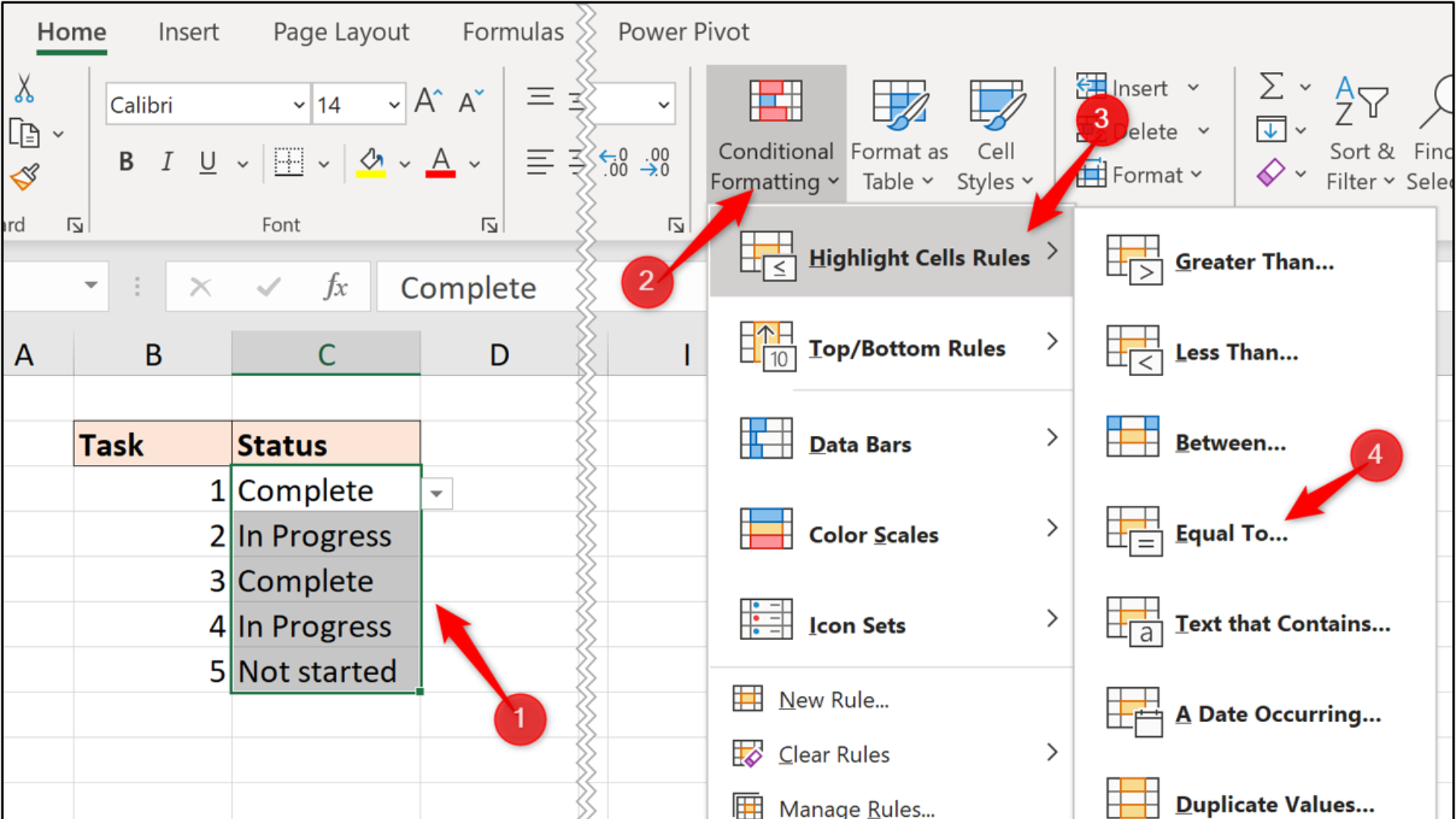
1. Select the Data Range

Highlight the range of cells you want to format. This can be a single column, row, or an entire table.

2. Open the Conditional Formatting Menu

Navigate to the 'Home' tab, then click on 'Conditional Formatting' in the 'Styles' group. A dropdown menu will reveal various formatting options.

3. Choose a Formatting Rule

Depending on your data and objectives, select the appropriate rule. It could be data bars, colour scales, icon sets, or custom formulas.

4. Define Formatting Conditions

Specify the conditions under which the formatting should be applied. This could involve setting thresholds, values, or formulas.

5. Preview and Apply Formatting

Before finalising, use the preview feature to see how your formatting will appear. Once satisfied, click 'OK' to apply the formatting to the selected cells.

Advanced Tips and Tricks

Custom Formulas for Complex Conditions

Sometimes, the built-in formatting rules won't cover your specific needs. Custom formulas allow you to tailor the formatting to your precise requirements. For instance, you can use a formula to highlight cells containing a specific combination of values.

Gradient Scales with Data Bars

Experiment with gradient scales in data bars for more nuanced insights. Instead of simple colours, the length of the data bar can represent the magnitude of the data, providing a deeper understanding.

Customising Conditional Formatting

Font, Border, and Fill Colour Customization

Conditional formatting extends beyond colours. You can also customise font styles, borders, and fill colours to ensure a cohesive and appealing data presentation.

Avoiding Common Mistakes

Consistency is Key

Maintain a consistent approach to formatting across your data. Using too many colours or icons can confuse your audience and dilute the impact of the visual cues.

Effective Troubleshooting

Formatting might not always behave as expected. If you encounter issues, double-check your conditions and formulas. Clear and specific rules prevent unintended outcomes.

Conclusion

As you embark on your journey of mastering Excel conditional formatting, remember that XL Intelligence is here to guide you. By following our tips, examples, and step-by-step instructions, you'll harness the full potential of this powerful feature. Turn data from an overwhelming mass into a clear, insightful presentation. Elevate your data visualisation game today and bring your insights to life!

Ready to take your data presentation to the next level? Contact us at XL Intelligence for expert guidance on unleashing the true potential of Excel's conditional formatting.

For personalised assistance and to learn more about Excel's advanced features, visit our contact page and get in touch with our Excel experts today!