Welcome to our comprehensive guide on Excel Pivot Tables, where we'll show you how to master data analysis like a pro in just five easy steps! As experts in Excel-based solutions, we, at XL Intelligence, understand the power and significance of Pivot Tables in transforming raw data into valuable insights. Whether you're a beginner or an experienced user, this tutorial will equip you with the skills to harness the full potential of Excel Pivot Tables.

Understanding Excel Pivot Tables

Excel Pivot Tables are a fundamental tool for data analysis that allows you to summarise, analyse, and interpret large datasets quickly and efficiently. These tables provide a dynamic way to organise, filter, and present data, making it easier to identify trends, patterns, and outliers. By leveraging Pivot Tables, you can gain valuable insights from your data without the need for complex formulas or lengthy manual calculations.

Step 1: Data Preparation

Before diving into Pivot Table creation, it's crucial to ensure your data is well-prepared. Imagine a scenario where I was working on a sales data analysis project, and I neglected to clean the dataset properly. The result? My Pivot Table displayed inaccurate figures and misleading conclusions. So, I quickly learned the importance of cleaning, sorting, and formatting data before proceeding.

To begin, organise your data in a tabular format with clear headings for each column. Remove any duplicates, errors, or irrelevant information. Additionally, ensure that your data is free from empty cells or missing values, as these can affect the accuracy of your analysis.

Step 2: Creating a Pivot Table

Once your data is organised, it's time to create your Pivot Table. In Excel, you can use the PivotTable Wizard or utilise the newer 'PivotTable Recommended' option for a more intuitive experience. The latter automatically suggests Pivot Tables based on your data, streamlining the process significantly.

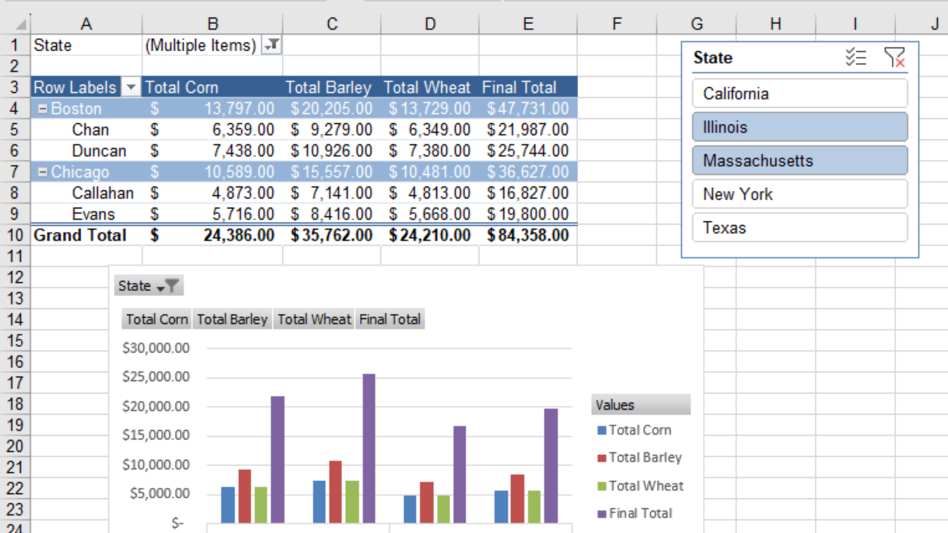
To create a Pivot Table, select your dataset, click on the 'Insert' tab, and choose 'PivotTable' from the options. Excel will guide you through the setup, allowing you to choose where you want to place the table and which fields to include. You can drag and drop fields into the rows, columns, and values areas to structure your Pivot Table effectively.

Step 3: Choosing the Right Fields

Choosing the right fields for your Pivot Table is critical to obtain meaningful insights. Think of it like selecting ingredients for a recipe; each field adds a unique flavor to your analysis. In the context of our 'longtail keyword' (Excel pivot table tutorial), let's consider our sales data analysis example.

For this scenario, I chose the 'Product Category' as the row field, 'Salesperson' as the column field, and 'Sales Amount' as the value field. This setup allowed me to observe how different salespeople performed in each product category, helping identify top performers and opportunities for improvement.

Step 4: Analysing Data with Pivot Tables

Now that your Pivot Table is set up, it's time to dive into data analysis. Excel offers various functionalities, such as filtering, sorting, and calculated fields, to help you analyse your data effectively.

Filtering data allows you to focus on specific subsets of information, such as a particular product category or sales region. Sorting helps you arrange data in ascending or descending order, providing insights into top-selling products or highest-earning salespeople. Calculated fields enable you to perform custom calculations, such as calculating profit margins or average sales per salesperson.

Step 5: Customising and Presenting Results

The appearance of your Pivot Table plays a crucial role in presenting your findings to stakeholders. Excel offers a range of customisation options to make your Pivot Table visually appealing and easy to interpret.

You can format the table, change fonts, apply colors, and add borders to enhance readability. Additionally, incorporating charts and graphs helps you visualise trends and patterns more effectively. By creating a combination of Pivot Tables and charts, I was able to present a comprehensive sales performance report that impressed both my team and management.

Advanced Tips and Tricks

For those looking to take their Excel Pivot Table skills to the next level, there are various advanced tips and tricks to explore. One such technique is creating a Pivot Chart, which updates automatically whenever you refresh your Pivot Table data. This dynamic integration between Pivot Tables and Pivot Charts further simplifies data visualisation and analysis.

You can also explore Power Pivot, an Excel add-in that extends Pivot Table capabilities by enabling data modeling and handling large datasets. Additionally, learn how to leverage calculated fields and measures effectively to derive more complex insights.

Conclusion

Excel Pivot Tables are undoubtedly a powerful tool for data analysis, enabling you to unlock valuable insights from your datasets. By following our five easy steps, you can confidently navigate through Pivot Table creation, data analysis, and presentation like a pro.

Whether you're analysing sales data, financial information, or any other dataset, mastering Pivot Tables is a skill that can significantly impact your decision-making process. So, let us, at XL Intelligence, help you on your data-driven journey. Visit our contact page to learn more about our Excel-based solutions and how we can support your business in harnessing the true potential of Pivot Tables.